AQI - Build Your Data Skills by Analyzing AQI of Different Indian Cities

[aupreti]

Follow the instructions given to do your very first data analysis and understand more about Air Pollution and AQI

Instructions For Doing the Analysis
A )Setting Up the Work Sheet

1. Right Click on the Data tab and duplicate the sheet
   
   

2. Click on the plus button on the left corner and add a new tab
   
   

3. Rename it to “Analysis”

B) First Anlaysis

1. Click on “Insert” from Top Menu
2. Click on “Pivot Table”
3. In “Create pivot table” click on the “Select data range” icon on the right -
4. Enter the range - ”Copy of Data!A1:L11510”
5. Tick mark “Existing sheet” in “Insert to” and click on “Select data range” icon on the right
6. Enter the location - “Analysis!A1”
7. Click on “ Create”
8. In the “Pivot table editor”, go to “Rows” and add “Month”
9. Un- check the “Show total” checkbox
10. Go to “Columns” add “Year”
11. Un- check the “Show total” checkbox
12. Go to “Values” add “AQI”
13. In “AQI”, go to “Summarise by”, and select “AVERAGE”
14. Go to “Filters” add “City”
15. In the “City”, go to “ Showing all items” and Select only “Delhi”
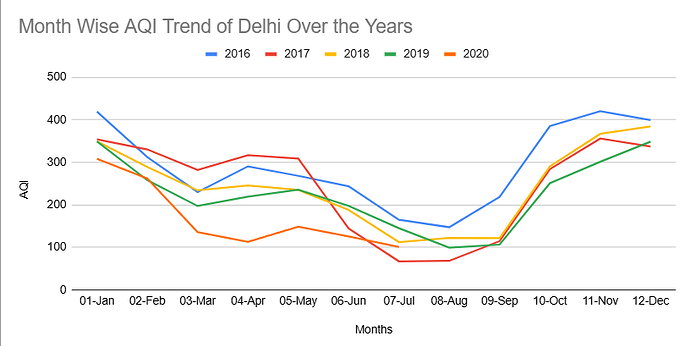
16. The Table is showing the Month Wise Average AQI of Delhi over multiple years
17. Click on “Insert” from Top Menu and click on “Chart”
18. In the “Chart Editor” tab on the right, select “Line chart” as “Chart type”
19. In “Data Range’’, click on the icon the right to select data range
20. Select “A2:F14” as the data range and click “OK”
21. Scroll down and tick mark “Use row 2 as headers”